Plato’s Theory of Forms contains the idea that all objects have an abstract ‘form’; an underlying ‘essence’ shared by all objects of a certain type. By Plato’s theory, all horses have an innate ‘horseness’ despite differences in outward appearance, and all apples have a distinct ‘appleness’ that lets us group a Granny Smith and a Red Delicious into a single ‘apple’ category. Extending this idea to human faces, all faces would have a shared, abstract structure called ‘faceness’.
There are arguments against Plato’s theory, but it still invites an interesting analogy with an idea in machine learning called eigenfaces. Could we use machine learning to uncover abstract, common parts underlying a human face?
Let’s start with face images. Is there an abstract form or a set of common, abstract ingredients shared by all faces? If there are, how could we use these common ingredients to construct two completely different faces?
This post will look into these questions, and although it may not reach definitive conclusions about Platonic forms, it does contain some pretty cool gifs at the end. We’ll use a machine learning technique called principal component analysis (PCA) and apply it to a dataset of face images.
By using PCA, we can represent data in lower dimensions by expressing it as a combination of its most ‘important’ directions. In the space of face images, these ‘important’ directions are called eigenfaces. Intuitively, each of the eigenfaces explains some of the variance between face images. Once we compute the eigenfaces, we can use them to compactly represent and reconstruct the original face images.
To perform the investigation, our tools will be Python, numpy, and scipy. All of the code, as well as some sample results, can be found on GitHub.
Representing the Images
The first step is preparing the images. First, we choose one image of each person from the faces94 dataset, and convert it to greyscale. By converting to greyscale, each pixel in the image can be represented as a single number. We represent the entire image set as an n x p matrix X, with n images and p pixels; each row of the matrix corresponds to an image’s pixels.
X = numpy.array([imread(i, True).flatten() for i in jpgs])
Performing PCA
Now, with the images loaded comes the core of the work: performing the principal component analysis. First, we find the mean face image and subtract it from each face in the dataset. This centers the data at the origin.
# compute the mean face
mu = numpy.mean(X, 0)
# mean adjust the data
ma_data = X - mu
SVD
Now, we decompose the mean-centered matrix into three parts using singular value decomposition (SVD). SVD decomposes the face matrix into three parts, UΣV, where U and V are the left and right singular vectors of X, respectively, and Σ is a diagonal matrix whose elements are the singular values of X.
U, S, V = linalg.svd(ma_data.transpose(), full_matrices=False)
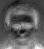
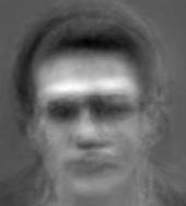
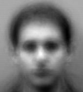
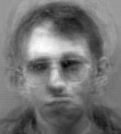
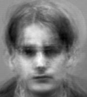
Now, the columns of U form an orthonormal basis for the eigenspace of X‘s covariance matrix. What significance does this have for our investigation? Each column of U is a singular vector, corresponding to an eigenface! The corresponding singular values are found in Σ, and are decreasing from left to right. Visually, here are the first three columns of U, which are the first three eigenfaces:
How Many Eigenfaces?
Our dataset consists of only n = 117 training images, and each image has p = 180*200 = 36,000 pixels. Since n < p we observe that SVD will return only n eigenfaces with non-zero singular values; therefore we have n = 117 different eigenfaces.
Hauntingly Important Faces
The eigenfaces are abstract – and scary – faces. Intuitively, we can think of each eigenface as an ‘ingredient’ common to all faces in the dataset. A person’s face is constructed using some combination of the eigenface ingredients. In fact, all of the faces in X contain some amount of each eigenface- perhaps these ingredients are the abstract, common structure we were looking for!
Some eigenfaces are more ‘important’ to reconstructing faces than others. The columns of U are ordered in terms of decreasing importance, since their corresponding singular values in Σ decrease from left to right. The first column, corresponding to the first eigenface, is the most ‘important’; it explains the most variance in the space of faces. The second column, corresponding to the second eigenface is the second most ‘important’, the third column, corresponding to the the third eigenface is the third most ‘important’, and so on.
The first eigenface:
is more important than the 103rd eigenface:
We can reconstruct a face by using these eigenface ingredients; each face is just a weighted combination of the ingredients. We obtain the weights by dotting the mean centered data with the eigenfaces:
# weights is an n x n matrix
weights = numpy.dot(ma_data, e_faces)
For each image, we have a weight for each of the n eigenfaces, so weights is an n x n matrix. To reconstruct a face, we dot the face’s weights (a row in the weights matrix) with the transpose of the eigenfaces (n x p matrix), and add the mean face back in:
# reconstruct the face located at img_idx
recon = mu + numpy.dot(weights[img_idx, :], e_faces.T)
We’ve reconstructed a face by dotting the face’s weights with each eigenface. But how is this useful? Let’s consider what we used to reconstruct the image:
- a p x n matrix of eigenfaces (e_faces)
- a n x 1 vector of weights (one row from weights)
The eigenfaces matrix stays constant for all reconstructions; to reconstruct a new face we simply supply a weight vector. Therefore a face is uniquely defined by a n x 1 vector. Keep in mind that n = 117 and p = 36000; instead of using all 36000 pixels to distinguish one image from another, we now only use 117 weights!
But it gets better; in fact we’ve yet to fully take advantage of PCA’s dimensionality reduction. So far, we have reconstructed the face using all n weights and n eigenfaces. However, we observed that the initial eigenfaces explain more variance between faces than the later eigenfaces.
Leaner Reconstruction
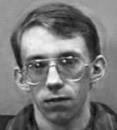
We can take advantage of this observation, and remove the ‘unimportant’ eigenfaces; instead of using all n, we can instead use just the first k weights and eigenfaces, where k < n. By doing so we’re representing the face image using fewer dimensions, and we can reconstruct an approximation of the face using only this lower-dimensional data. To illustrate, let’s choose k = 50 and reconstruct the image:
# reconstruct the image at img_idx using only 50 eigenfaces
k = 50
recon = mu + numpy.dot(weights[img_idx, 0:k], e_faces[:, 0:k].T)
This time, to reconstruct the image all we needed was (keeping in mind that k < p):
- a p x k matrix of eigenfaces (k columns of e_faces)
- a k x 1 vector of weights (k columns of one row from weights)
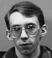
However, the picture indicates a tradeoff: the fewer eigenfaces we use, the rougher the reconstruction, and the more eigenfaces we use, the closer we get to the original picture. In other words, when we reduce k, we give up some reconstruction accuracy. But this is where eigenfaces get fascinating. Since each eigenface is less and less important to the reconstruction, we reach something resembling the original picture fairly quickly; in our case it’s never necessary to use all 117 eigenfaces! To illustrate, let’s consider the following image.
The original image is:
The image reconstructed using only 1 eigenface is:
k = 1
recon = mu + numpy.dot(weights[img_idx, 0:k], e_faces[:, 0:k].T)
It’s still very abstract.
Using 20 eigenfaces, we have:
k = 20
recon = mu + numpy.dot(weights[img_idx, 0:k], e_faces[:, 0:k].T)
The picture is becoming more accurate; we can begin to make out his glasses, hair, and face shape.
At just 40 eigenfaces, we already have a picture that is clearly the same individual that we started with:
And at 50:
Reconstructing another person’s face, we have:
It’s fascinating that the eigenfaces stay the same from person to person; we simply change the k weightings and have a new identity. Again, if we just store one copy of the eigenfaces matrix, we can reconstruct a person’s picture using just k numbers. We can also compare two faces using just k dimensions instead of p.
To further illustrate the idea, here are some animations. The animations start with the mean face, then progressively reconstruct a face, using an increasing number of eigenfaces. Specifically, each frame uses one eigenface more than the previous frame. At first we see massive changes from frame to frame, since the early eigenfaces are the most informative. Towards the end we see that using an additional eigenface only makes a minor change; more eigenfaces are being used, but the face looks roughly the same.
Back to the Forms
We began with a vague search for an abstract, common ‘form’ for face images. By computing eigenfaces, we created a set of shared ‘ingredients’ that define face images. Starting from an abstract image (the mean face), we are able to add combinations of the ingredients to reconstruct completely different faces.
Perhaps we could interpret the eigenfaces as defining the underlying, abstract ‘faceness’ in each face image. The same procedure could be applied to pictures of apples to visualize ‘appleness’, or pictures of horses for ‘horseness’.
Regardless, eigenfaces are a great intuition-builder and a fascinating way to visualize PCA. Eigenfaces have applications in facial recognition, and the more general PCA has a vast range of applications throughout machine learning.
Credits
This post was inspired by Jeremy Kun’s eigenface post on his great blog, Math ∩ Programming, Penn Machine Learning lecture notes, and a presentation about eigenfaces. The dataset used was discussed in Kun’s post, and is found here.


